Introduction E9F5FC

Questions FFFFC0

• View
• Edit
• History
• Print

Hamiltonians and Quantum Symmetries

Michael Stone, Ching-Kai Chiu, Abhishek Roy. Symmetries, Dimensions, and Topological Insulators: the mechanism behind the face of the Bott clock.

Interpretations

• Hamiltonian is the self. It describes what it means to have a coherent self-identity that can evolve in time. It is the agglomeration of all of the dynamical possibilities for a system which can experience particular conditions.
• A nonordinary symmetry on a Hamiltonian means that it has a context. Metaphysically, a context is very restricted because we can think of the context of the context, which inverts it. Inverting a context returns it to what is known ({$+1$}) or to its opposite, what is not known {$-1$}. The context functions like the dual of a vector space and so taking the dual of the dual takes us back to the vector space (the set of all possibilities that it could have satisfying the constraints) but here we end up with two options, not just one.
• The {$O(n)\times O(n)$} and likewise stages mean that the number of positive energy states and negative energy states have to match up. This is the same as matching up what is known and what is not known, or being and not being. Consciousness is responsible for lining this up. And this allows us to proceed to the next stage.

Observations

Hamiltonians are Hermitian.

The {$m\in\frak{m}_i$} are commuting with {$J_1,\dots,J_m$} but anticommuting with {$J_{m+1}$}. This means that they branch away from those that commute with all {$J_i$}. Thus they are all disjoint. And the initial {$m\in\frak{m}_0$} are those that simply anticommute with {$J_1$}. What does it mean for them to commute with a mythical {$J_0$} and previous linear complex structures?

Two ways of looking at the Lie group embeddings

• There is a linear complex structure {$J_i$} and the matrices it commutes with form a subgroup {$H$} of {$G$}.
• There is a Lie algebra {$\frak{g}=\frak{h}+\frak{m}$} where {$[\frak{h},\frak{h}]\in\frak{h}, [\frak{h},\frak{m}]\in\frak{m}, [\frak{m},\frak{m}]\in\frak{h}$}, and {$\frak{m}$} are {$i\times$} the Hamiltonians (corresponding to the time evolution operators {$e^{iHt/ \hbar}$} in the unitary group), and {$G$} and {$H$} are the Lie groups corresponding to {$\frak{g}$} and {$\frak{h}$}.

The symmetric spaces form a sequence of order-parameter spaces that arise as we progressively break a large symmetry by introducing more and more symmetry-breaking operators. As a bonus, the matrices representing the symmetry-breaking operators will later serve as the building blocks of model Hamiltonians that yield all possible topologically non-trivial band structures.

These Hamiltonians are maps between complex vectors spaces and so are the quantum symmetries. {$C$} and {$T$} are antilinear maps.

In Stone, Chiu, Roy, the antilinear maps {$\mathcal{C}H\mathcal{C}^{-1} = −H$} can be understood as real matrices with {$2\times 2$} antilinear blocks. They are given by complex matrices {$CH^∗ C^{−1} = −H$}.

---

---

---

Quantum symmetries

The symmetries are of the form {$J_i$}, squaring to {$-I$}, or {$J_iJ_jJ_k$}, squaring to {$+I$}.

{$C$} is either {$J_2$} or {$J_2J_4J_6=N=\varphi$} (establishing real structure). Note that both are based on {$D=\textrm[1,-1,1,-1]$} but {$C$} has {$D$} in the upper triangular matrix and {$-D$} in the lower triangular matrix, whereas {$N$} has {$D$} in the top half of the diagonal followed by {$-D$} in the bottom half. Note also that {$-D$} is simply reading {$D$} in the reverse order.

{$J_2=\begin{pmatrix} & & 1 & & & & & \\ & & & -1 & & & & \\ -1 & & & & & & & \\ & 1 & & & & & & \\ & & & & & & 1 & \\ & & & & & & & -1 \\ & & & & -1 & & & \\ & & & & & 1 & & \\ \end{pmatrix}$}

{$J_2J_4J_6=\begin{pmatrix} 1 & & & & & & & \\ & -1 & & & & & & \\ & & 1 & & & & & \\ & & & -1 & & & & \\ & & & & -1 & & & \\ & & & & & 1 & & \\ & & & & & & -1 & \\ & & & & & & & 1 \\ \end{pmatrix}$}

{$J_4J_6=\begin{pmatrix} & & -1 & & & & & \\ & & & -1 & & & & \\ 1 & & & & & & & \\ & 1 & & & & & & \\ & & & & & & 1 & \\ & & & & & & & 1 \\ & & & & -1 & & & \\ & & & & & -1 & & \\ \end{pmatrix}$}

{$T$} is based on the {$J_i$} which anticommutes with {$m\in\frak{m}$}. Thus it is either {$J_1$}, {$J_2$}, {$J_3$} or it ends in {$J_5,J_6,J_7$}. It skips over {$J_4$} and {$J_8$}, which yield isometries.

{$J_2=C$} when {$m$} anticommutes with {$J_2$} and then {$J_2=T$} when {$m$} anticommutes with {$J_3$}. Similarly, {$J_2J_4J_6=C$} when {$m$} anticommutes with {$J_6$} and then {$J_2J_4J_6=T$} when {$m$} anticommutes with {$J_7$}.

---

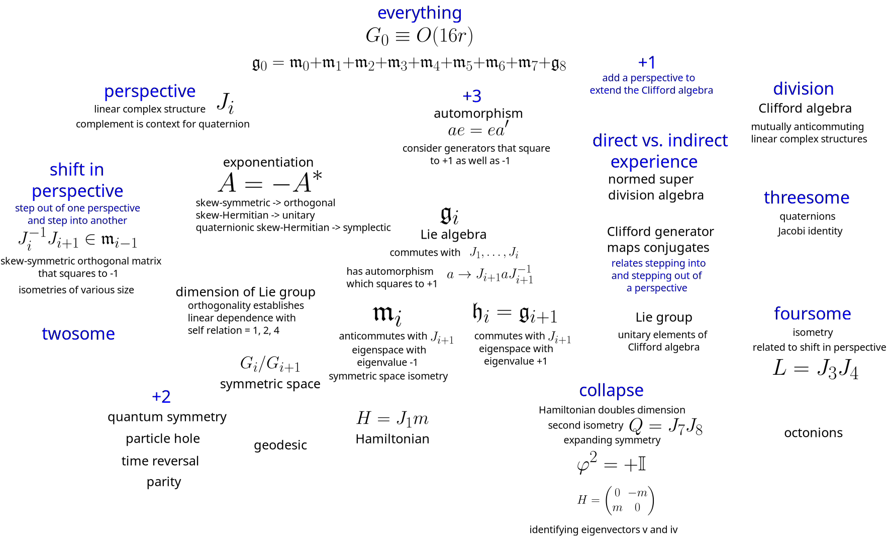
{$D≡ O(16r)$}: The coset generators {$m ∈ m_{−1}$} are real skew-symmetric matrices. These are not diagonalizable within the reals. We need to double the Hilbert space to {$R^{32r}$} and tensor with “{$i$}”= {$−iσ_2$} so that the Hamiltonian becomes {$H = −iσ_2 ⊗ m$}. Then taking {$\phi = σ_3 ⊗ I$} to be the real structure that defines complex conjugation, we have {$ϕH = −Hϕ$}. This {$\phi$} therefore defines a particle-hole symmetry that squares to {$+I$}. We should not count the eigenvectors {$v$} and {$iv ≡ (−iσ_2 ⊗ I)v$} as being distinct. (We can regard the {$R^{32r}$} space and the operators {$“i$}” and {$ϕ$} as being inherited from the previous cycle of the Bott clock.)

“{$i$}” {$=\begin{pmatrix} 0 & -1 \\ 1 & 0 \\ \end{pmatrix}=-i\sigma_2=-i\begin{pmatrix} 0 & -i \\ i & 0 \\ \end{pmatrix}$}

{$m^T=-m$} is a {$16\times 16$} matrix.

{$H = −iσ_2 ⊗ m = \begin{pmatrix} 0 & -m \\ m & 0 \\ \end{pmatrix}$} is a {$32\times 32$} matrix.

{$σ_3= \begin{pmatrix} 1 & 0 \\ 0 & -1 \\ \end{pmatrix}$}

{$\phi=σ_3 ⊗ I=\begin{pmatrix} I & 0 \\ 0 & -I \\ \end{pmatrix}$} is a {$32\times 32$} real matrix that is the antilinear map that defines complex conjugation

{$\phi H = \begin{pmatrix} I & 0 \\ 0 & -I \\ \end{pmatrix}\begin{pmatrix} 0 & -m \\ m & 0 \\ \end{pmatrix} = \begin{pmatrix} 0 & -m \\ -m & 0 \\ \end{pmatrix} = \begin{pmatrix} 0 & m \\ -m & 0 \\ \end{pmatrix}\begin{pmatrix} I & 0 \\ 0 & -I \\ \end{pmatrix} = -H\phi$}

{$\phi^2=I$}

For particle hole symmetry, we think here in terms of real antilinear {$\phi$} rather than complex matrix {$C$}.

Let eigenvector {$v=\begin{pmatrix}v_1 \\ v_2 \end{pmatrix}$} such that {$Hv=\lambda_v v$}. Then {$Hv=\begin{pmatrix} 0 & -m \\ m & 0 \\ \end{pmatrix}\begin{pmatrix}v_1 \\ v_2 \end{pmatrix}=\begin{pmatrix}-mv_2 \\ mv_1 \end{pmatrix}$} and so {$mv_2=-\lambda_v v_1$} and {$mv_1=\lambda_v v_2$}.

Define an equivalent eigenvector {$iv ≡ (−iσ_2 ⊗ I)v = \begin{pmatrix} 0 & -I \\ I & 0 \\ \end{pmatrix}\begin{pmatrix}v_1 \\ v_2 \end{pmatrix} = \begin{pmatrix}-v_2 \\ v_1 \end{pmatrix}$}. We have {$Hiv=\lambda_v iv$}. Thus {$Hiv=\begin{pmatrix} 0 & -m \\ m & 0 \\ \end{pmatrix}\begin{pmatrix}-v_2 \\ v_1 \end{pmatrix} = \begin{pmatrix}-mv_1 \\ -mv_2 \end{pmatrix} $} and so {$mv_1=\lambda_v v_2$} and {$mv_2=-\lambda_v v_1$}.

The eigenvector is the same in that it differs only by a (complex) scalar.

Given {$m(v_1+iv_2)=(a+bi)(v_1+iv_2)$} we have {$\lambda_v=i(a+bi)=-b+ai$} where {$H(v_1+iv_2)=i(a+bi)(v_1+iv_2)$}.

So set {$\begin{pmatrix}-v_2 \\ v_1 \end{pmatrix}\sim \begin{pmatrix}v_1 \\ v_2 \end{pmatrix}$}

---

{$DIII ≡ O(16r)/U(8r)$}: The {$m ∈ \frak{m}_0$} ’s are real skew symmetric matrices that anticommute with {$J_1$} . We can keep {$C = ϕ$} as a particle-hole symmetry and take {$T = ϕ ⊗ J_1$} as a time reversal that commutes with {$H = −iσ_2 ⊗ M$} and squares to {$−I$}. The product of {$C$} and {$T$} is {$J_1$} , and this a linear (commutes with {$−iσ_2 ⊗ I$}) “{$P$} ” type symmetry that anticommutes with {$H$}.

{$m$} consists of pairs of {$2\times 2$} blocks of the form {$\begin{matrix} & \begin{pmatrix} a & b \\ b & -a \\ \end{pmatrix} \\ \begin{pmatrix} -a & -b \\ -b & a \\ \end{pmatrix} & \\ \end{matrix}$} which together encode a quaternion of the form {$aj+bk$}. Separately, each block {$\begin{pmatrix} a & b \\ b & -a \\ \end{pmatrix}=\begin{pmatrix} a & -b \\ b & a \\ \end{pmatrix}\begin{pmatrix} 1 & 0 \\ 0 & -1 \\ \end{pmatrix}$} encodes multiplication by a complex number {$a+bi$} times a conjugation.

{$H = −iσ_2 ⊗ m = \begin{pmatrix} 0 & -m \\ m & 0 \\ \end{pmatrix}$} is a {$32\times 32$} matrix.

{$C=\phi=\begin{pmatrix} I & 0 \\ 0 & -I \\ \end{pmatrix}$} is a {$32\times 32$} matrix.

{$CH=\begin{pmatrix} I & 0 \\ 0 & -I \\ \end{pmatrix}\begin{pmatrix} 0 & -m \\ m & 0 \\ \end{pmatrix}=\begin{pmatrix} 0 & -m \\ -m & 0 \\ \end{pmatrix}$}

{$HC=\begin{pmatrix} 0 & -m \\ m & 0 \\ \end{pmatrix}\begin{pmatrix} I & 0 \\ 0 & -I \\ \end{pmatrix}=\begin{pmatrix} 0 & m \\ m & 0 \\ \end{pmatrix}=-CH$}

{$T = \phi ⊗ J_1$} This is true if we understand {$\phi$} as a {$2\times 2$} matrix and note that {$J_1$} is a {$16\times 16$} matrix. {$T= \begin{pmatrix} J_1 & 0 \\ 0 & -J_1 \\ \end{pmatrix} $} is a {$32\times 32$} matrix.

{$T^2=-I$}

{$TH=\begin{pmatrix} J_1 & 0 \\ 0 & -J_1 \\ \end{pmatrix}\begin{pmatrix} 0 & -m \\ m & 0 \\ \end{pmatrix}=\begin{pmatrix} 0 & -J_1m \\ -J_1m & 0 \\ \end{pmatrix}=\begin{pmatrix} 0 & mJ_1 \\ mJ_1 & 0 \\ \end{pmatrix}=\begin{pmatrix} 0 & -m \\ m & 0 \\ \end{pmatrix}\begin{pmatrix} J_1 & 0 \\ 0 & -J_1 \\ \end{pmatrix}=HT$}

{$P=J_1=CT=\begin{pmatrix} I & 0 \\ 0 & -I \\ \end{pmatrix} \begin{pmatrix} J_1 & 0 \\ 0 & -J_1 \\ \end{pmatrix}=\begin{pmatrix} J_1 & 0 \\ 0 & J_1 \\ \end{pmatrix}$} is a {$32\times 32$} matrix.

{$Pi=\begin{pmatrix} J_1 & 0 \\ 0 & J_1 \\ \end{pmatrix}\begin{pmatrix} 0 & -I \\ I & 0 \\ \end{pmatrix}=\begin{pmatrix} 0 & -J_1 \\ J_1 & 0 \\ \end{pmatrix} = \begin{pmatrix} 0 & -I \\ I & 0 \\ \end{pmatrix}\begin{pmatrix} J_1 & 0 \\ 0 & J_1 \\ \end{pmatrix}=iP$}

{$PH=\begin{pmatrix} J_1 & 0 \\ 0 & J_1 \\ \end{pmatrix}\begin{pmatrix} 0 & -m \\ m & 0 \\ \end{pmatrix}=\begin{pmatrix} 0 & -J_1m \\ J_1m & 0 \\ \end{pmatrix}$}

{$HP=\begin{pmatrix} 0 & -m \\ m & 0 \\ \end{pmatrix}\begin{pmatrix} J_1 & 0 \\ 0 & J_1 \\ \end{pmatrix}=\begin{pmatrix} 0 & -mJ_1 \\ mJ_1 & 0 \\ \end{pmatrix}=\begin{pmatrix} 0 & J_1m \\ -J_1m & 0 \\ \end{pmatrix}=-PH$}

Define {$J_1\equiv P$}

---

{$AII≡ U(8r)/Sp(4r)$}: The generators {$m ∈ \frak{m}_1$} are real skew matrices that commute with {$J_1$} and anticommute with {$J_2$} . They can be regarded as skew-quaternion-hermitian matrices with complex entries. We no longer need set {$i → −iσ_2 ⊗ I$} as the matrices no longer have elements coupling between the artificial copies. We instead use {$J_1$} as the surrogate for “{$i$}.” Now {$H = J_1 m$} is real symmetric, and commutes with {$T = J_2$} . This {$T$} acts as a time reversal operator squaring to {$−I$}.

{$\frak{g}_1$} are the {$8\times 8$} skew-Hermitian matrices. Their entries are complex numbers. The transpose of the imaginary numbers equals the matrix entries and the transpose of the real numbers equals {$-1$} times the matrix entries.

{$\frak{h}_1$} are {$4\times 4$} quaternionic skew-Hermitian matrices, which is to say, the matrices {$A=-A^Q$} where {$A^Q$} is the quaternionic conjugate transpose. Their entries are {$2\times 2$} matrices of {$2\times 2$} matrices which are either complex linear blocks (coding complex numbers) or antilinear blocks (of real numbers).

Specifically, consider the multiplication of a quaternion as a vector {$x_0 + x_1i + x_2j + x_3k$} times a quaternion {$a + bi + cj + dk$} as a matrix. We have four equations:

• {$x_0a -x_1b -x_2c -x_3d$} gives the real coefficient
• {$x_0b + x_1a + x_2d - x_3c$} gives the {$i$} coefficient
• {$x_0c - x_1d + x_2a + x_3b$} gives the {$j$} coefficient
• {$x_0d + x_1c -x_2b + x_3a$} gives the {$k$} coefficient

Thus we can express the quaternion {$a + bi + cj + dk$} as the matrix

{$\begin{pmatrix} a & b & c & d \\ -b & a & -d & c \\ -c & d & a & -b \\ -d & -c & b & a \\ \end{pmatrix}$}

This gives a way for coding the quaternions that extends {$i$} with {$-i$} and yields a matrix of complex numbers. Here {$a=1$} codes for the identity, {$b=1$} codes for {$i$}, {$c=-1$} codes for {$j$} and {$d=1$} codes for {$k$} as in Stone, Chiu, Roy, and we can express them together in terms of {$2\times 2$} complex linear matrices X and Y

{$\begin{pmatrix} X & -Y \\ \bar{Y} & \bar{X} \\ \end{pmatrix}$}

Note that when {$a=0$}, this matrix, understood in terms of complex numbers, is skew-Hermitian. Note also that the imaginary components are given by skew-symmetric real matrices.

Furthermore, when {$a=0$} and {$c=0$}, this matrix is skew-hermitian with regard to the quaternion conjugate transpose.

Crucially, given a skew-hermitian matrix, consider a {$2\times 2$} matrix within it. It is either off the diagonal or on the diagonal.

If it is off the diagonal, then consider

{$\begin{pmatrix} a & b & c & d \\ -b & a & -d & c \\ -c & d & a & -b \\ -d & -c & b & a \\ \end{pmatrix}$},

its negative complex conjugate transpose {$\begin{pmatrix} -a & b & c & d \\ -b & -a & -d & c \\ -c & d & -a & -b \\ -d & -c & b & -a \\ \end{pmatrix}$}

and its negative quaternionic conjugate transpose {$\begin{pmatrix} -a & b & c & d \\ -b & -a & -d & c \\ -c & d & -a & -b \\ -d & -c & b & -a \\ \end{pmatrix}$} which is the same.

If the matrix is on the diagonal, then being skew-hermitian we must have {$a=0$}, so consider

{$\begin{pmatrix} 0 & b & c & d \\ -b & 0 & -d & c \\ -c & d & 0 & -b \\ -d & -c & b & 0 \\ \end{pmatrix}$}

Again, it is furthermore skew-hermitian with regard to the quaternionic conjugate transpose if and only if {$c=0$}.

Now consider the {$4\times 4$} real matrices which are complex linear, that is, their {$2\times 2$} blocks can be identified with complex numbers. Consider when they commute or anticommute with the matrix {$J_2$} that encodes the quaternion {$j$}. Note that the {$j$} are on the diagonal and so the commuting or anticommuting {$4\times 4$} blocks can be anywhere. Namely, we are dealing with {$\sum_{k=k}j_{kk}a_{kl}=ja_{kl}=\pm a_{lk}j=\sum_{k=k}a_{lk}j_{kk}$}.

{$J_2=j=\begin{pmatrix} & & 1 & \\ & & & -1 \\ -1 & & & \\ & & 1 & \\ \end{pmatrix} = \begin{pmatrix} 0 & r \\ -r & 0 \\ \end{pmatrix}$}

{$\begin{pmatrix} 0 & r \\ -r & 0 \\ \end{pmatrix}\begin{pmatrix} c_{11} & c_{12} \\ c_{21} & c_{22} \\ \end{pmatrix} = \begin{pmatrix} rc_{21} & rc_{22} \\ -rc_{11} & -rc_{12} \\ \end{pmatrix}$}

{$\begin{pmatrix} c_{11} & c_{12} \\ c_{21} & c_{22} \\ \end{pmatrix}\begin{pmatrix} 0 & r \\ -r & 0 \\ \end{pmatrix} = \begin{pmatrix} -c_{12}r & c_{11}r \\ -c_{22}r & c_{21}r \\ \end{pmatrix}$}

If they commute, then {$rc_{11}=-c_{22}r$}, {$rc_{21}=-c_{12}r$}, thus {$rc_{11}r^{-1}=-c_{22}$}, {$rc_{21}r^{-1}=-c_{12}$}, thus {$\overline{c_{11}}=c_{22}$}, {$\overline{c_{12}}=-c_{21}$}, yielding the quaternion

{$\begin{pmatrix} X & Y \\ -\overline{Y} & \overline{X} \\ \end{pmatrix}$}

Whereas if they anticommute, we have what Stone, Chiu, Roy call the skew-quaternion

{$\begin{pmatrix} X & Y \\ \overline{Y} & -\overline{X} \\ \end{pmatrix}$}

Now {$\frak{g}_1=\frak{u}(8)$} are the {$8\times 8$} skew-Hermitian matrices and {$\frak{h}_1=\frak{sp}(4)$} are quaternion skew-Hermitian matrices and {$\frak{m}_1$} are skew-quaternion Hermitian matrices.

Exploring the latter, now consider

{$\begin{pmatrix} a & b & c & d \\ -b & a & -d & c \\ c & -d & -a & b \\ d & c & -b & -a \\ \end{pmatrix}$}

If it is on the diagonal, then since it is skew-Hermitian, it must be that {$a=0$}, {$c=0$} and {$d=0$}.

Multiplying by {$J_1$} gives

{$\begin{pmatrix} & -1 & & \\ 1 & & & \\ & & & -1 \\ & & 1 & \\ \end{pmatrix}\begin{pmatrix} 0 & b & 0 & 0 \\ -b & 0 & 0 & 0 \\ 0 & 0 & 0 & b \\ 0 & 0 & -b & 0 \\ \end{pmatrix} = \begin{pmatrix} b & 0 & 0 & 0 \\ 0 & b & 0 & 0 \\ 0 & 0 & b & 0 \\ 0 & 0 & 0 & b \\ \end{pmatrix}$}

which is a block {$bI$} in a real symmetric Hamiltonian.

Off the diagonal, {$m$} has blocks {$\begin{pmatrix} a & b & c & d \\ -b & a & -d & c \\ c & -d & -a & b \\ d & c & -b & -a \\ \end{pmatrix}$} with negative complex conjugate transposes {$\begin{pmatrix} -a & b & -c & -d \\ -b & -a & d & -c \\ -c & d & a & b \\ -d & -c & -b & a \\ \end{pmatrix}$}

Multiplying by {$J_1$} gives

{$\begin{pmatrix} & -1 & & \\ 1 & & & \\ & & & -1 \\ & & 1 & \\ \end{pmatrix}\begin{pmatrix} a & b & c & d \\ -b & a & -d & c \\ c & -d & -a & b \\ d & c & -b & -a \\ \end{pmatrix} = \begin{pmatrix} b & -a & d & -c \\ a & b & c & d \\ -d & -c & b & a \\ c & -d & -a & b \\ \end{pmatrix}$}

and

{$\begin{pmatrix} & -1 & & \\ 1 & & & \\ & & & -1 \\ & & 1 & \\ \end{pmatrix}\begin{pmatrix} -a & b & -c & -d \\ -b & -a & d & -c \\ -c & d & a & b \\ -d & -c & -b & a \\ \end{pmatrix} = \begin{pmatrix} b & a & -d & c \\ -a & b & -c & -d \\ d & c & b & -a \\ -c & d & a & b \\ \end{pmatrix}$}

Taken together the pair of blocks are part of a real symmetric Hamiltonian {$H=J_1m$}. They code quaternions:

{$q=\begin{pmatrix}X & Y \\ -\overline{Y} & \overline{X} \\ \end{pmatrix}$} and {$\overline{q}=\begin{pmatrix}\overline{X} & -Y \\ -\overline{Y} & X \\ \end{pmatrix}$}

Thus the Hamiltonian {$H$} is its own quaternionic conjugate transpose {$H^Q=H$}.

{$T^2=-I$}

{$HT=J_1mJ_2=J_1(-J_2m)=J_2J_1m=TH$}

Define {$J_2\equiv T$}

Alternatively, consider the multiplication of a quaternion {$a + bi + cj + dk$} as a matrix times a quaternion {$x_0 + x_1i + x_2j + x_3k$} as a vector. We have four equations:

• {$ax_0 - bx_1 - cx_2 - dx_3$} gives the real coefficient
• {$bx_0 + ax_1 - dx_2 + cx_3$} gives the {$i$} coefficient
• {$cx_0 + dx_1 + ax_2 - bx_3$} gives the {$j$} coefficient
• {$dx_0 - cx_1 + bx_2 + ax_3$} gives the {$k$} coefficient

Thus we can express the quaternion {$a + bi + cj + dk$} as the matrix

{$\begin{pmatrix} a & -b & -c & -d \\ b & a & -d & c \\ c & d & a & -b \\ d & -c & b & a \\ \end{pmatrix}$}

Note that here the complex number {$i$} is extended with {$-i$}. Here {$a=1$} codes for the identity, {$b=1$} codes for {$i$}, {$c=-1$} codes for {$j$} and {$d=-1$} codes for {$k$}. We can express this matrix in terms of {$2\times 2$} real matrices which encode a complex linear matrix L and an antilinear map A

{$\begin{pmatrix} L & -A \\ A & L \\ \end{pmatrix}$}

Note that the imaginary components are given by skew-symmetric real matrices.

---

{$CII≡ Sp(4r)/Sp(2r) × Sp(2r)$}: The matrices {$m ∈ \frak{m}_2$} commute with {$J_1$} and {$J_2$} but anti- commute with {$J_3$}. Again {$H = J_1 m$}. We can set {$T = J_3$} as this commutes with with {$H$} and squares to {$−I$}. {$P = J_2 J_3$} anticommutes with {$H$} but commutes with {$J_1$} (and so is a linear map) while {$C = J_2$} anticommutes with {$H$}, is antilinear and squares to {$−I$}.

The Lie algebra {$\frak{g}_2=\frak{sp}(4r)$} consists of matrices {$M$} with quaternionic ({$4\times 4$} real) entries such that {$M^Q=-M$}.

Furthermore the {$8\times 8$} matrices {$m$} anti-commmute with {$J_3$}. We consider

{$\begin{pmatrix}q_{11} & q_{12} & q_{13} & q_{14} \\ q_{21} & q_{22} & q_{23} & q_{24} \\ q_{31} & q_{32} & q_{33} & q_{34} \\ q_{41} & q_{42} & q_{43} & q_{44} \\ \end{pmatrix} \begin{pmatrix}-k & & & \\ & k & & \\ & & -k & \\ & & & k \\ \end{pmatrix} = \pm\begin{pmatrix}-k & & & \\ & k & & \\ & & -k & \\ & & & k \\ \end{pmatrix} \begin{pmatrix}q_{11} & q_{12} & q_{13} & q_{14} \\ q_{21} & q_{22} & q_{23} & q_{24} \\ q_{31} & q_{32} & q_{33} & q_{34} \\ q_{41} & q_{42} & q_{43} & q_{44} \\ \end{pmatrix}$}

{$\begin{pmatrix}-q_{11}k & q_{12}k & -q_{13}k & q_{14}k \\ -q_{21}k & q_{22}k & -q_{23}k & q_{24}k \\ -q_{31}k & q_{32} & -q_{33}k & q_{34}k \\ -q_{41}k & q_{42}k & -q_{43}k & q_{44}k \\ \end{pmatrix} = \pm \begin{pmatrix} kq_{11} & kq_{12} & kq_{13} & kq_{14} \\ -kq_{21} & -kq_{22} & -kq_{23} & -kq_{24} \\ kq_{31} & kq_{32} & kq_{33} & kq_{34} \\ -kq_{41} & -kq_{42} & -kq_{43} & -kq_{44} \\ \end{pmatrix}$}

Note that the quaternions {$q_{kl}$} are written with different matrices than the {$k$} in {$J_3$}. We have

{$\begin{pmatrix} a & b & c & d \\ -b & a & -d & c \\ -c & d & -a & -b \\ -d & -c & b & -a \\ \end{pmatrix}\begin{pmatrix} & & & 1 \\ & & 1 & \\ & -1 & & \\ -1 & & & \\ \end{pmatrix} = \begin{pmatrix} -d & -c & b & a \\ -c & d & a & -b \\ b & a & d & -c \\ a & -b & -c & -d \\ \end{pmatrix} $}

{$\begin{pmatrix} & & & 1 \\ & & 1 & \\ & -1 & & \\ -1 & & & \\ \end{pmatrix}\begin{pmatrix} a & b & c & d \\ -b & a & -d & c \\ -c & d & -a & -b \\ -d & -c & b & -a \\ \end{pmatrix} = \begin{pmatrix} -d & -c & b & -a \\ -c & d & -a & -b \\ b & -a & d & -c \\ -a & -b & -c & -d \\ \end{pmatrix} $}

We have {$qk=kq$} implies {$a=0$} whereas {$qk=-kq$} implies {$b=c=d=0$}.

Let {$r_{ij}$} be real quaternions and {$s_{ij}$} be imaginary quaternions. We have that

{$\begin{pmatrix} s_{11} & r_{12} & s_{13} & r_{14} \\ r_{21} & s_{22} & r_{23} & s_{24} \\ s_{31} & r_{32} & s_{33} & r_{34} \\ r_{41} & s_{42} & r_{43} & s_{44} \\ \end{pmatrix}$} commute with {$J_3$} and are the matrices in {$\frak{g}_2$} that are in {$\frak{h}_2$}.

{$\begin{pmatrix} r_{11} & s_{12} & r_{13} & s_{14} \\ s_{21} & r_{22} & s_{23} & r_{24} \\ r_{31} & s_{32} & r_{33} & s_{34} \\ s_{41} & r_{42} & s_{43} & r_{44} \\ \end{pmatrix}$} anticommute with {$J_3$} and are the matrices in {$\frak{g}_2$} that are in {$\frak{m}_2$}.

{$H=J_1m$}

{$T=J_3= \begin{pmatrix} & & & -1 & & & & \\ & & -1 & & & & & \\ & 1 & & & & & & \\ 1 & & & & & & & \\ & & & & & & & 1 \\ & & & & & & 1 & \\ & & & & & -1 & & \\ & & & & -1 & & & \\ \end{pmatrix}$}

{$TH=J_3J_1m=J_1mJ_3=HT$}

{$C=J_2$}

{$CH=J_2J_1m=-J_1mJ_2$}

{$P=CT=J_2J_3$}

{$PJ_1=J_2J_2J_1=J_1J_2J_3=J_1P$}

{$PH=J_2J_3J_1m=J_1J_2J_3m=-J_1J_2mJ_3=-J_1mJ_2J_3=-HP$}

Define {$J_3\equiv T$}

---

{$C≡ {Sp(2r) × Sp(2r)}/Sp(2r) ≃ Sp(2r)$}: The matrices {$m ∈ \frak{m}_3$} commute with {$J_1 , J_2 , J_3$} , and anticommute with {$J_4$} , and we can restrict ourselves to the subspace in which {$K = J_1 J_2 J_3$} takes a definite value, say {$+1$}. The Hamiltonian {$J_1 m$} commutes with {$J_4$} – but {$J_4$} does not commute with {$J_1 J_2 J_3$} and so is not allowed as an operator on our subspace. Indeed no product involving {$J_4$} is allowed. But {$C = J_2$} commutes with {$J_1 J_2 J_3$} and still anticommutes with {$H$}. Thus we still have a particle-hole symmetry squaring to {$−1$}. The old time reversal {$J_3$} now anticommutes with {$H$} and looks like another particle- hole symmetry, but is not really an independent one as in this subspace {$J_3 = J_2 J_1$} and {$J_1$} is simply multiplication by “{$i$}.”

Continue with the results from before and ask what commutes and anticommutes with {$J_4$}

{$\begin{pmatrix} s_{11} & r_{12} & s_{13} & r_{14} \\ r_{21} & s_{22} & r_{23} & s_{24} \\ s_{31} & r_{32} & s_{33} & r_{34} \\ r_{41} & s_{42} & r_{43} & s_{44} \\ \end{pmatrix}\begin{pmatrix} & k & & \\ k & & & \\ & & & k \\ & & k & \\ \end{pmatrix} = \begin{pmatrix} r_{12}k & s_{11}k & r_{14}k & s_{13}k \\ s_{22}k & r_{21}k & s_{24}k & r_{23}k \\ r_{32}k & s_{31}k & r_{34}k & s_{33}k \\ s_{42}k & r_{41}k & s_{44}k & r_{43}k \end{pmatrix}$}

{$\begin{pmatrix} & k & & \\ k & & & \\ & & & k \\ & & k & \\ \end{pmatrix} \begin{pmatrix} s_{11} & r_{12} & s_{13} & r_{14} \\ r_{21} & s_{22} & r_{23} & s_{24} \\ s_{31} & r_{32} & s_{33} & r_{34} \\ r_{41} & s_{42} & r_{43} & s_{44} \\ \end{pmatrix} = \begin{pmatrix} kr_{21} & ks_{22} & kr_{23} & ks_{24} \\ ks_{11} & kr_{12} & ks_{13} & kr_{14} \\ kr_{41} & ks_{42} & kr_{43} & ks_{44} \\ ks_{31} & kr_{32} & ks_{33} & kr_{34} \end{pmatrix} $}

Recall that {$r_{ij}=-\overline{r_{ji}}$} and {$s_{ij}=-\overline{s_{ji}}$} where we are applying the quaternionic conjugate transpose. This means that on the diagonal these real quaternions are {$0$} when the matrix is commuting with {$J_4$}.

More generally, consider {$r_{ij}k=kr_{mn}$}. The real quaternions are scalars and this yields {$r_{ij}=r_{mn}$} when the matrix commutes with {$J_4$} and {$r_{ij}=-r_{mn}$} when they anticommute.

As regards {$s_{ij}k=ks_{mn}$}, note that

{$\begin{pmatrix} & 1 \\ -1 & \\ \end{pmatrix}\begin{pmatrix} X & Y \\ -\overline{Y} & \overline{X} \\ \end{pmatrix} = \begin{pmatrix}\overline{X} & \overline{Y} \\ -Y & X \\ \end{pmatrix}$} is the complex conjugate. Note also that for imaginary quaternions the conjugate is simply the negative.

Thus the blocks of the form {$\begin{pmatrix} s & r \\ r' & s' \\ \end{pmatrix} $} become {$\begin{pmatrix} s & r \\ r & -s \\ \end{pmatrix} $} if the matrix commutes with {$J_4$} and become {$\begin{pmatrix} s & r \\ -r & s \\ \end{pmatrix} $} if the matrix anticommutes with {$J_4$}.

{$H=J_1m$}

Restrict to {$8$}-dimensional {$V_+=[v_1,v_2,v_3,v_4,0,0,0,0,v_9,v_{10},v_{11},v_{12},0,0,0,0]$} for {$16$}-dimensional operator {$J_1J_2J_3 = \textrm{diag}[1,1,1,1,-1,-1,-1,-1]$}. This is the same as restricting to a two-dimensional quaternionic vector space {$V_+=[q_1,q_2]$}. This means that each {$2\times 2$} block of quaternions gets reduced to the quaternion {$(s)$}.

Note that reducing the vector space eliminates the distinction between those {$m$} which commute with {$J_4$} and those that don't.

{$m=\begin{pmatrix} s_{11} & s_{13} \\ s_{31} & s_{33} \\ \end{pmatrix} =\begin{pmatrix} s_{11} & s_{13} \\ -\overline{s_{13}} & s_{33} \\ \end{pmatrix}$} for {$m^Q=-m$} and recall that the {$s_{ij}$} are imaginary quaternions.

{$H=J_1m=\begin{pmatrix} is_{11} & is_{13} \\ -i\overline{s_{13}} & is_{33} \\ \end{pmatrix}$} where {$i$} is the quaternion {$i_2$}.`

{$HJ_4=J_1mJ_4=J_4J_1m=J_4H$}

{$J_4K=J_4J_1J_2J_3=-J_1J_2J_3J_4=-KJ_4$}

{$C=J_2$}

{$CK=J_2J_1J_2J_3=-J_1J_2J_2J_3=J_1J_2J_3J_2=KC$}

{$CH=J_2J_1m=-J_1J_2m=-J_1mJ_2=-HC$}

In this halved subspace we now have the relation {$J_3=J_1J_2$} which functions like {$J_3=iJ_2$}.

We also don't have operators which include {$J_4$} because they would have to be built with {$J_1, J_2, J_3$} but these all commute with {$K=J_1J_2J_3$}. However, the matrices {$m$} do anticommute with {$J_4$}, which is how its impact is felt. It restricts the matrices {$m$}.

---

{$CI≡ Sp(2r)/U(2r)$}: The {$m ∈ \frak{m}_4$} anticommute with {$J_5$} . Now {$J_4 J_5$} commutes with {$J_1 J_2 J_3 $}, and so is an allowed operator. It anticommutes with {$H = J_1 m$} and commutes with {$J_1$} . It is therefore a “{$P$} ”-type linear map. The map {$T = J_2 J_4 J_5$} is antilinear (anticommutes with {$J_1$} ), commutes with {$H$} and {$T^2 = +I$}. We can take {$C = J_2$} again.

{$m=\begin{pmatrix} s_2 & \\ & s_2 \\ \end{pmatrix}$} where {$s_2=\begin{pmatrix} d & & & -c \\ & d & c & \\ & -c & d & \\ c & & & d \\ \end{pmatrix}$} is made of complex linear {$2\times 2$} blocks.

{$H = J_1 m = \begin{pmatrix} i_4s_2 & \\ & i_4s_2 \\ \end{pmatrix}$} where {$i_4s_2=\begin{pmatrix} & -d & -c & \\ d & & & -c \\ -c & & & -d \\ & -c & d & \\ \end{pmatrix}$}

{$C=J_2$}

{$T=J_2J_4J_5=\begin{pmatrix} & & & 1 & & & & \\ & & 1 & & & & & \\ & 1 & & & & & & \\ 1 & & & & & & & \\ & & & & & & & -1 \\ & & & & & & -1 & \\ & & & & & -1 & & \\ & & & & -1 & & & \\ \end{pmatrix}$}

{$P=J_4J_5=-CT=\begin{pmatrix} & -1 & & & & & & \\ 1 & & & & & & & \\ & & & 1 & & & & \\ & & -1 & & & & & \\ & & & & & 1 & & \\ & & & & -1 & & & \\ & & & & & & & -1 \\ & & & & & & 1 & \\ \end{pmatrix}$}

{$PK=KP$}

---

{$AI ≡ U(2r)/O(2r)$}: The {$m ∈ \frak{m}_5 n$} anticommute with {$J_6$} , and we are to restrict ourselves to the subspace on which {$K = J_1 J_2 J_3 = +1$} and {$M = J_1 J_4 J_5 = +1$}. The map {$T = J_3 J_4 J_6$} commutes with {$K$} and {$M$} and commutes {$H = J_1 m$}. We have {$T^2 = +I$}. We could equivalently take {$T = J_2 J_4 J_6$}.

{$H=J_1m$}

{$T=N=J_2J_4J_6=\textrm{diag}[-1,1,-1,1,-1,1,-1,1]$}

---

{$BDI≡ O(2r)/O(r) × O(r)$}: The {$m ∈ \frak{m}_6$} anticommute with {$J_7$} , and we are to restrict our- selves to the eigenspaces of {$K = J_1 J_2 J_3 , M = J_1 J_4 J_5$} . The {$m$} also commute with the antilinear operator {$N = J_2 J_4 J_6$} which we can regard as our real structure {$ϕ$}. We therefore set {$C = ϕ = N$}. Now {$J_3 J_4 J_7 , J_3 J_5 J_6 , J_2 J_5 J_7$} and {$J_1 J_6 J_7$} all commute with {$K$}, {$M$} and {$N$}, each squaring to {$+I$}. In the restricted subspace {$J_3 J_4 J_7 ∝ J_2 J_5 J_7 ∝ J_1 J_6 J_7$} and {$J_3 J_5 J_6 ∝ I$}. The problem here is what to take for “{$i$},” as the current {$H → J_1 m$} will take us out of the eigenspace of {$N$}. But this is the problem we started with. We need to double the space and keep “{$i$}”= {$J_1$} and the real structure {$ϕ = N$}. We are therefore retaining the {$R^{2r}$} Hilbert space. With {$H = J_1 m$} we have that {$T = J_1 J_6 J_7$} commutes with {$H$} and squares to {$+I$}.

I don't understand how {$T=J_1J_6J_7$} and {$H=J_1 m$} commute. I get {$TH=J_1J_6J_7J_1m=J_1^2J_6J_7m=-J_1mJ_1J_6J_7=-HT$}.

---

{$D≡ {O(r) × O(r)}/O(r) ≃ O(r)$}: Now the {$m ∈ \frak{m}_7$} anticommute with {$J_8$} and, except for the factor “{$i$}”= {$J_1$} , we should stay in the space where {$K = J_1 J_2 J_3 , M = J_1 J_4 J_5 , N = J_2 J_4 J_6$} and {$P = J_1 J_6 J_7$} take the value {$+1$} With {$H = J_1 m$} we have that {$C = ϕ = N$} anticommutes with {$H$}, and brings us full circle.

We have
{$K=J_1J_2J_3=\textrm{diag}[-1,-1,-1,-1,1,1,1,1]$}
{$M=J_1J_4J_5=\textrm{diag}[-1,-1,1,1,-1,-1,1,1]$}
{$N=J_2J_4J_6=\textrm{diag}[-1,1,-1,1,-1,1,-1,1]$}
{$P=J_1J_6J_7=\textrm{diag}[\hat{r},\hat{r},-\hat{r},-\hat{r},\hat{r},\hat{r},-\hat{r},-\hat{r}]$}
{$Q=J_7J_8=\textrm{diag}[\hat{i},\hat{i},\hat{i},\hat{i},\hat{i},\hat{i},\hat{i},\hat{i}]$} where

{$\hat{r}=\begin{pmatrix}1 & 0\\0 & -1\\ \end{pmatrix}, \hat{i}=\begin{pmatrix}0 & -1\\1 & 0\\ \end{pmatrix}$}

The {$16$}-dimensional vector space on which {$K,M,N,P$} take the value {$+1$} is {$(0,0,0,0,0,0,0,0,0,0,0,0,0,0,0,s)$}.

{$O(1)=\{(1),(-1)\}$} and we can think of this in terms of {$2\times 2$} matrices expressing {$O(1)\times O(1)/O(1)$}

{$\begin{pmatrix} 1 & 0 \\ 0 & 1 \\ \end{pmatrix}$}, {$\begin{pmatrix} -1 & 0 \\ 0 & -1 \\ \end{pmatrix}$} are the values for {$m ∈ \frak{m}_7$}

{$H=J_1m$} has values {$\begin{pmatrix} 0 & -1 \\ 1 & 0 \\ \end{pmatrix}$}, {$\begin{pmatrix} 0 & -1 \\ 1 & 0 \\ \end{pmatrix}$} which expresses {$\pm i$}.

{$J_8= \begin{pmatrix} & & & & \hat{i}\hat{r} & & & \\ & & & & & -\hat{i}\hat{r} & & \\ & & & & & & -\hat{i}\hat{r} & \\ & & & & & & & \hat{i}\hat{r} \\-\hat{i}\hat{r} & & & & & & & \\ & \hat{i}\hat{r} & & & & & & \\ & & \hat{i}\hat{r} & & & & & \\ & & & -\hat{i}\hat{r} & & & & \\ \end{pmatrix}$}

---

读物

• Michael Stone. Gamma matrices, Majorana fermions, and discrete symmetries in Minkowski and Euclidean signature Appendix C. The {$C$} and {$T$} operations in Condensed Matter Systems.
• Ching-Kai Chiu, Jeffrey C. Y. Teo, Andreas P. Schnyder, Shinsei Ryu. Classification of topological quantum matter with symmetries
• Moore. Quantum Symmetries and Compatible Hamiltonians
• Moore. Quantum Symmetries and K-Theory.
• Alexei Kitaev. Periodic table for topological insulators and superconductors.
• Alexander Altland, Martin R. Zirnbauer. Nonstandard symmetry classes in mesoscopic normal-superconducting hybrid structures
• Jost Eschenburg. Lecture Notes on Symmetric Spaces.
• Jost Eschenburg. Geometry of Octonions.
• Shinsei Ryu, Andreas P Schnyder, Akira Furusaki, Andreas W W Ludwig. Topological insulators and superconductors: ten-fold way and dimensional hierarchy
• Adhip Agarwala, Arijit Haldar, Vijay B. Shenoy. The tenfold way redux: Fermionic systems with N-body interactions.
• Ludwig. Topological Phases: Classification of Topological Insulators and Superconductors of Non-Interacting Fermions, and Beyond.

Observations

• Note that a linear complex structure on a real vector space {$V$} is simply an automorphism on {$V$} that squares to the minus identity {$-I$}. This allows multiplication by complex scalars to be defined so that {$V$} is regarded as a complex vector space. Also, given {$J_i^2=-I$}, note that {$(J_i\otimes I)^2=J_i^2\otimes I^2=-I\otimes I$} and so I can do, as I have done, in defining {$J_i\otimes I$}.
• I should be careful to define {$J_i$} as a {$16\times 16$} matrix in {$O(16)$} not as I have done (tensoring the {$8\times 8$} matrix) but as the authors do.
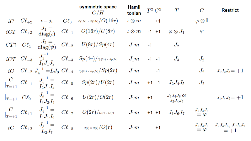
• The matrices {$m\in\frak{m}$} exist in a decomposition of a Lie algebra {$\frak{g}=\frak{h}+\frak{m}$} where {$\frak{h}$} is a Lie subalgebra of {$\frak{g}$}, and the corresponding Lie groups are {$G$} and {$H$}, with {$H$} a subgroup of {$G$}.
• We have that {$\frak{g}=\frak{m}_0+\frak{m}_1+\frak{m}_2+\dots + \frak{m}_7 + \frak{h}_7$} where {$\frak{g}$} and {$\frak{h}_7$} are essentially the same but in what way?
• The Lie algebra and Lie group are related by the exponential map {$\textrm{exp}:\frak{g}\rightarrow \;$}{$G$} given by {$\textrm{exp}(X)=\sum_{k=0}^\infty \frac{X^k}{k!}$}
• The Lie algebra of the orthogonal group {$O(n)$} consists of the real skew-symmetric {$n \times n$} matrices (for which the transpose is the negative)(the multiplicative inverse gets understood as the additive inverse).
• The Lie algebra of the unitary group {$U(n)$} consists of the {$n \times n$} skew-Hermitian matrices (for which the conjugate transpose is the negative of the matrix)(the multiplicative inverse gets understood as the additive inverse).
• The Lie algebra of the symplectic group {$Sp(n)$} consists of {$n \times n$} quaternionic skew-Hermitian matrices (for which the quaternionic conjugate transpose is the negative of the matrix)(the multiplicative inverse gets understood as the additive inverse).
• In all cases, the negative (real, conjugate, quaternionic conjugate) transpose, the real numbers on the diagonal are zero, the real numbers change sign when transposed, and the imaginary numbers are transposed without change in sign.
• The real skew-symmetric matrices have imaginary eigenvalues. Multiplying the matrices by "i" (and what does that mean?) gives them real eigenvalues. That gives us the Hamiltonian, which gives us physical insight.
• The matrices {$m\in\frak{m}_i$} commute with {$J_1,\dots ,J_i$} and anticommute with {$J_{i+1}$}.
• The matrices in {$\frak{m}_i$} are defined by the vector space decomposition {$\frak{g}_i=\frak{g}_{i+1}\oplus\frak{m}_i$} where {$[\frak{m}_i,\frak{m}_i]\subset \frak{g}_{i+1}$} and {$[\frak{m}_i,\frak{g}_{i+1}]\subset \frak{m}_{i+1}$}.
• Once the matrices can be understood to have complex entries (they don't have antilinear entries), then we can define multiplication by {$i$} within that context. Otherwise, we need to establish a broader context for making sense of multiplication by {$i$}.
• The {$J_k$} are {$16\times 16$} matrices whereas the matrices {$m$} and the Hamiltonian change in size.
• The Hamiltonian is understood as a complex matrix, that is, a matrix with complex entries.
• The quaternionic matrix relates the key four operators as {$2\times 2$} blocks: the identity, the two antilinear operators, and the linear operator which is their product.
• I want to understand how anti-commuting operators and commuting operators complement each other. The anti-commuting operators pair to yield commuting operators, so the anti-commuting operators are odd and the commuting operators are even. The anti-commmuting operators yield the matrices {$\frak{m}$} in the decomposition of the Lie algebra whereas the commuting operators yield the group {$H$} and the lie subalgebra {$\frak{h}$} so I have to stay mindful of the distinction between the Lie group and the Lie algebra.
• {$JM=MJ$} implies {$e^JM=Me^J$}. But {$JM=-MJ$} implies {$e^JM=Me^{-J}$}.
• The matrices are {$32\times 32$} precisely when particle hole (charge conjugation) symmetry, the complex matrix {$C$} or the antilinear real matrix {$\phi$} squares to {$+I$}.
• A Hamiltonian {$J_1m$} is a real symmetrix matrix and thus is Hermitian and has real eigenvalues. There is a real orthogonal matrix {$Q$} such that {$D=Q^TJ_1mQ$} is a diagonal matrix.
• A real {$n\times n$} matrix {$A$} is symmetric if and only if {$ \left< Ax,y\right>= \left< x,Ay\right> \; \forall x,y\in \mathbb{R}^n$}

Ideas

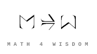
• Each {$m_i$} forms a context for the {$i+1$}st perpsective. In the orthogonal case {$O(16r)$}, it forms a context for {$1$}, the zeroth perspective. Then {$O(16r)/U(8r)$} yields {$\frak{m}_1$} as the quaternions of the form {$aj + bk$}, which establishes a context for the quaternions of the form {$ci$}. It is forming a context for {$\frak{h}_i=\frak{g}_{i+1}$}. Consider how these contexts are framing or evoking the octonionic generators.
• Orthogonal, unitary, symplectic form a threesome (the two out of three rule) whereby two of them ground the third as a shift-in-perspective.
• Cycling through all 8 contexts makes something holistic, incorporating all possibilities, balancing them, creating the conditions for consciousness.
• Why is H the same as -H? Perhaps upon doubling the matrices some vectors have to be identified and then perhaps in those circumstances H and -H match up. Perhaps this is the basis for contradiction. For it was all based on the assumption that H and -H are distinguished.
• The three operations should express themselves in Bott periodicity. Operation +1 expresses the application of a linear complex structure. Operation +2 expresses quantum symmetries. Operation +3 can describe movement in the opposite direction, the swap squaring to +1, which is like three steps at once, as with an operator {$iJ_1$}. It may also relate the operations +1 and +2.
• Can keeping distinct a particle and anti-particle be considered a symmetry? I think it is a trivial symmetry that can be made explicit.
• Particle hole symmetry expands the Hamiltonians because it maps the Hamiltonian to the negative Hamiltonian with conjugation, mapping particles to holes and vice versa.
• The operation +2. How does it express itself with these quantum symmetries?
• Time reversal symmetry distinguishes between whether the mind is all totally filled up or whether it is the complement, what is left over, the twosome, which relates the two minds.
• Introspection has a maximum of 6 perspectives and the Clifford algebra Cl_{0,6} is all filled up when you have 8x8 matrices. But then you extend it by equating particles with anti-particles.
• Look at the {$C^2$} and the {$T^2$} as characterizing the divisions of everything. Two independent symmetries give an odd division, a single independent symmetry gives an even division.
• When charge conjugation squares to -1 then it is creating a realm of four possibilities, the foursome. So that is squeezed in between the {$T^4=1$} and the {$T$}.
• There are two kinds of symmetries - constraining and broadening - and particle hole symmetry is broadening for it equates a particle and a hole. Time reversal is a constraining symmetry. If you multiply the broadening symmetry by itself to get +1 then the expansion collapses. Whereas if you square and get -1, then it distinguishes the perspectives of the hole on that and the particle on that and that enriches the geometry, and this is more constraining, and this is all in the charge conjugation.
• Charge conjugation is 0 versus 4, it doesn't have the notion of complementing, except perhaps 4 is the average between 0 and 8. Whereas charge conjugation has 2 and 6 as complements, where 2 is the shift in perspective in terms of what is, and 6 in terms of what is not, what is missing.
• When the particle hole squares to +1, there is no extra geometry. When it squares to -1 it implies there is a greater geometry, the spin geometry, and that means that the symmetry was broader than you thought. And so then the particle hole symmetry is not adding more than what it does when there is no geometry, in the +1 case. But with time reversal it should be the other way around, that squaring to -1 is less constraining than squaring to +1.
• Particle hole symmetry is not a constraining symmetry but a broadening symmetry, it expands what a particle means, in the case of the orthogonal group it is the most free. I have to think about time reversal.
• Consider charge conjugation as describing 0 and 4, nullsome and foursome, and charge conjugation as relating 2 and 6, existence and morality, and when you put them together you average and that gives the numbers (for the divisions of everything).
• There are three choices that make for the eightfold contexts: negative or not, conjugate or not, transpose or not.
• Think of the dimensions of the orthogonal matrices as units of time. So as you go through the entire cycle you have used up units of time (the dimension has gone down from 16r to r) but otherwise you are back to where you started from.
• Lie groups are based on symmetries thus on distances, but the concept of distance changes, as grounded by symmetric spaces. For example, the metric for the orthogonal group, with which we start, yields a linear complex structure {$J_1$}, a perspective in a division of everything, which is compatible with the symplectic group, even though it has a different concept of distance. This leads from one concept of distance to another. Whereas the unitary group has a different concept of distance and relates to {$iJ_1$}.
• I expect that Bott periodicity is grounded in the dimensions of the Lie groups as given by the number of independent variables given by the orthogonality equations as given by the relevant norm - orthogonal, unitary, symplectic - and what it means that the notion of distance and orthogonality changes as we go from one to the other, as led by the linear complex structures.
• Hamiltonian accords with a single quasiparticle, thus its identity which takes up various perspectives. The Hamiltonian is restricted to an ever more elaborate surface described by a sequence of symmetry breakings and the identity is identified with one of the perspectives described.
• The Hamiltonian describes the experience of a self, a quasiparticle, free fermion, and it is related to a skew-symmetric matrix, which relates two Clifford algebra generators, the input and output, and maps all the possible shifts in perspective. Among these shifts in perspective you get yields zones. A distinguished shift in perspective takes one dynamical system to another dynamical system, without a way back, as with free will and fate.
• For each symmetric space check which versions of {$J_1$} commute and don't commute and figure out the logic for that.
• In U(2n) you can embed two copies U(n)xU(n) and take a diagonal U(n) and that embedding is driven by {$iJ_1$}. Similarly, you can do that for O(2n) and for Sp(2n) but that is driven by {$J_1$}, and if you keep going you get real Bott periodicity.

A Hamiltonian is specific to a single quasiparticle and that accords with an identity that takes up perspectives. As J_i are applied the Hamiltonian is restricted to an ever more elaborate surface and that quasiparticle, that "eye", is related to one of the possiblities (perspectives) in that sophisticated structure.

A 2x2 swap matrix {$ir$} swaps axes but doesn't indicate their orientation, it doesn't have to, whereas a rotation {$i$} swaps axes but also indicates an orientation to the axes. So that is an important distinction.

In the field of computational neuroscience, random matrices are increasingly used to model the network of synaptic connections between neurons in the brain. Dynamical models of neuronal networks with random connectivity matrix were shown to exhibit a phase transition to chaos[24] when the variance of the synaptic weights crosses a critical value, at the limit of infinite system size. Results on random matrices have also shown that the dynamics of random-matrix models are insensitive to mean connection strength. Instead, the stability of fluctuations depends on connection strength variation[25][26] and time to synchrony depends on network topology.

---