Math 4 Wisdom. "Mathematics for Wisdom" by Andrius Kulikauskas.

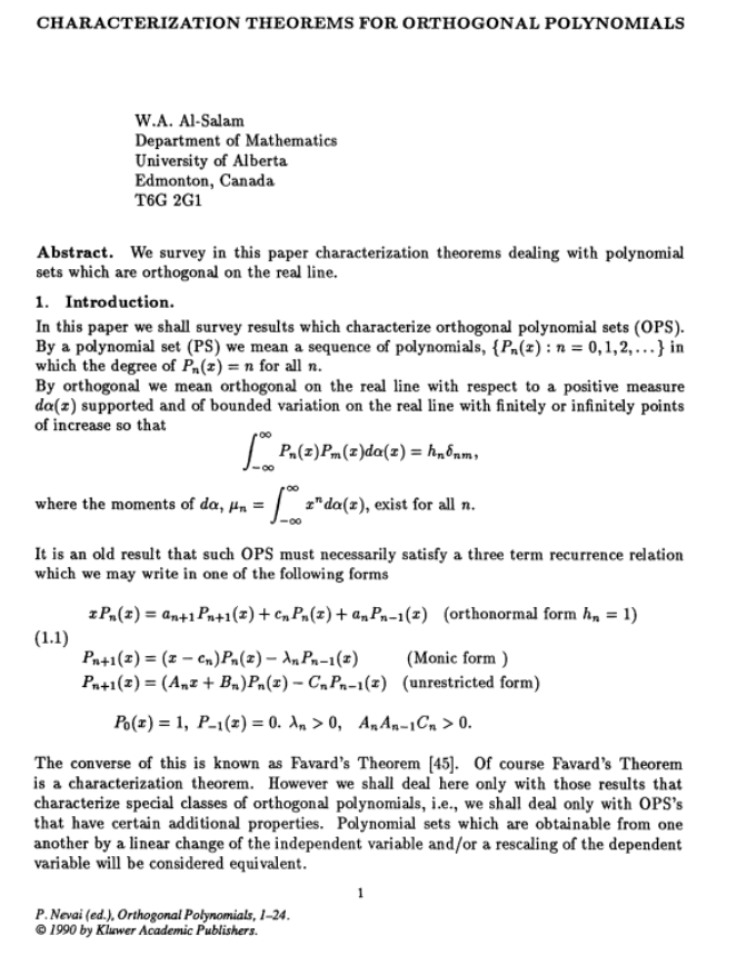
I am learning, contemplating and writing up a derivation of the classification of Sheffer polynomials.

Here are steps in the derivation.

Preliminaries

Understand what are orthogonal polynomial sets.

The coefficients of the polynomials are presumably rational numbers.

A polynomial set is a sequence of polynomials {$\{P_n(x):n=0,1,2...\}$} in which the degree of {$P_n(x)=n$} for all {$n$}. Polynomial sets are considered equivalent if they are obtainable from each other by a linear change of the independent variable {$x$} and/or a rescaling of the dependent variable (What is meant by dependent variable?)

A polynomial set is orthogonal with respect to a positive measure {$\textrm{d}\alpha$} if {$\int_{-\infty}^{\infty}P_n(x)P_m(x)\textrm{d}\alpha(x)=h_n\delta_{nm}$} where the moments {$\mu_n$} of {$\textrm{d}\alpha$}, {$\mu_n=\int_{-\infty}^{\infty}x^n\textrm{d}\alpha$}, exist for all {$n$}.

Understand the significance of orthogonal polynomials

How do orthogonal polynomials express the spectral theorem? If A is Hermitian, there exists an orthonormal basis of V consisting of eigenvectors of A. Each eigenvalue is real.

Recurrence relation

This recurrence relation for orthogonal polynomials is derived by expressing {$xP_n(x)$} in terms of the orthogonal polynomials as they form a basis for all polynomials. We observe that {$xP_n(x)$} has degree {$n+1$} and thus the expression cannot have any terms of higher degree. Nor can it have any terms of degree {$k<n-1$} as can be seen by linearizing {$xP_n(x)P_k(x)$}, which must yield {$0$}.

{$x$} is the quantum. Thus it is meaningful to focus on {$xP_n(x)$} and thus contemplate the following expression:

{$$xP_n(x) = P_{n+1}(x) + A_n P_n(x) + B_n P_{n-1}(x)$$}

Quadratic fetters for exponentials

{$P_n{x}$} does not depend on terms lower than {$n-2$}. This apparently imposes a quadratic growth on what otherwise could be growing exponentially in size and complexity.

Consider...

{$\int P_n(x)P_k(x) d\alpha = c_k\delta_{nk}$}
{$f(x)=f_0P_0(x)+f_1P_1(x)+\cdots+f_{n-1}P_{n-1}(x)$}
{$\int P_n(x)f(x) d\alpha = 0$}
look at {$\int xP_n(x)P_k(x) d\alpha$} This becomes an argument about {$P_n$}, and it says suppose that {$n\geq k$}, then because {$xP_k(x)$} has degree {$k+1$}, so if {$n>k+1$}, which means {$n-1 > k$}, then it will be {$0$}.

We get thus a chain where each polynomial is related to the polynomials directly above and below. This gives a way of thinking about a Dynkin diagram (especially their chains) in terms of raising operators {$x$} and lowering operators {$\frac{\textrm{d}}{\textrm{dx}}$}. A raising operator adds a new cell. A lowering operator removes any one of the existing {$n$} cells, thus marking it.

Recurrence relation

We can then make evident the recurrence relation:

{$$P_{n+1}(x) = (x - A_n) P_n(x) - B_n P_{n-1}(x)$$}

This is like climbing a ladder with a left foot on the rung below and the right foot on the rung below that. Your weight can be on either foot or both.

Weights and moments

Given a weight, it is possible to calculate its moments. Then the orthogonal polynomials associated to the weight can be calculated by a determinant of the moments.

This suggests why the combinatorics of orthogonal polynomials are based on permutations and their statistics. I should investigate that.

It also shows that the problem of classifying orthogonal polynomials is really the matter of classifying the weights by which the originate. The weight is the relevant space.

I found Chihara's, Viennot's and Kim and Zeng's combinatorial interpretations of the moments.

Sheffer Polynomials

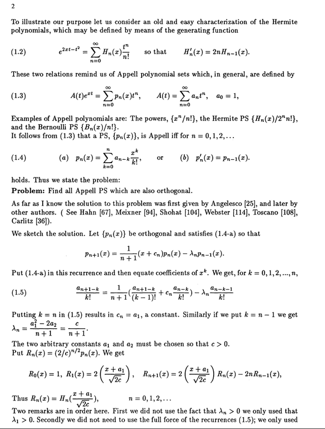
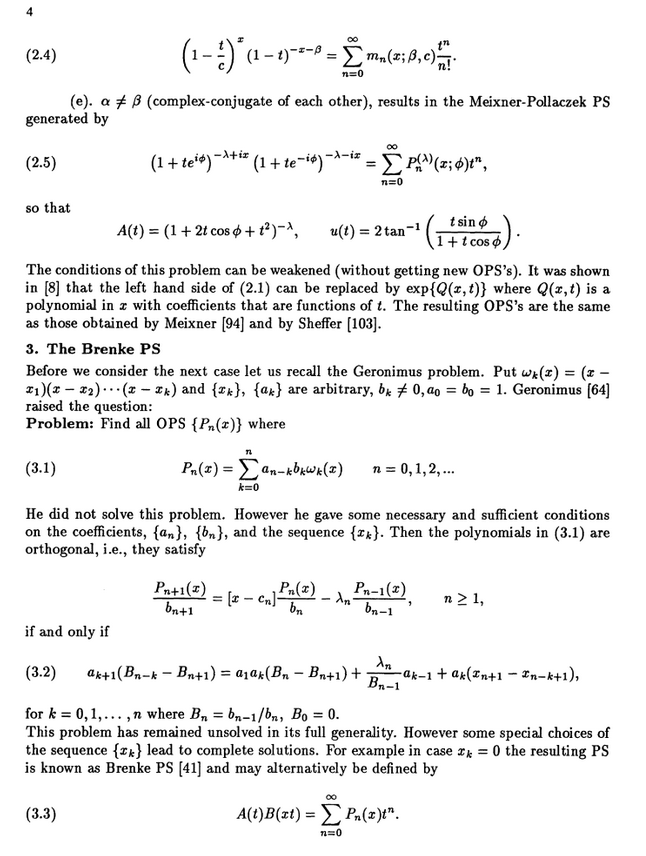
I want to classify orthogonal polynomial sets {$\{P_n(x)\}$} of the form

{$$\sum_{n=0}^{\infty}P_n(x)t^n=A(t)e^{xu(t)}$$}

where {$A(t)=\sum_{n=0}^{\infty}a_nt^n$}, {$a_0=1$}, and {$u(t)=\sum_{n=0}^{\infty}u_nt^n$}, {$u_0=0$}, {$u_1=1$}.

The generating function {$e^{xu(t)}$} is precisely that for polynomials of binomial type. The coefficients are precisely those given by Bell polynomials on scalars {$a_1, a_2, \cdots$} so that {$p_n(x)=\sum_{k=1}^{n=\infty}B_{n,k}(a_1,\cdots,a_{n-k+1})x^k$}. Furthermore, if we set {$P(t)=\sum_{n=1}^{\infty}\frac{a_n}{n!}t^n$}, then {$P^{-1}(\frac{\textrm{d}}{\textrm{dx}})$} is the delta operator of this sequence.

The form {$A(t)e^{xu(t)}$} is consequential in that it establishes an additional constraint above and beyond orthogonality which, working together, the two constraints yield very narrow possibilities. This form is remarkably constricting in how it links together the various powers of {$x$} and {$t$} when combined with orthogonality. Perhaps this is because orthogonality is a quadratic relationship, and here it is being combined with an exponential relationship. The weights are exponential, they have an analytic symmetry, they are reproduced by differentiation, along with an additional factor, and they overwhelm any polynomial factors as we go out to infinity. The quadratic constraint is a general theme, as with the tridiagonality of the Jacobi operator. I suspect the same theme is behind the restrictiveness of the Dynkin diagrams, which could be understood as chains of dimensions on which raising and lowering operators act. A might exponential horse is fettered by quadratic orthogonal shackles which keep one leg from extending too far from another.

Elements of Lie groups and Lie algebras

How does {$A(t)e^{xu(t)}$} relate to Lie groups and Lie algebras?

Lie group: The exponential map The exponential map from the Lie algebra to the Lie group is not always onto, even if the group is connected (though it does map onto the Lie group for connected groups that are either compact or nilpotent)
Exponential map (Lie theory) If G is compact, it has a Riemannian metric invariant under left and right translations, and the Lie-theoretic exponential map for G coincides with the exponential map of this Riemannian metric.
For {$X$} in {$\mathfrak{g}$}, there is a unique Lie group homomorphism {$t\rightarrow\textrm{exp}(tX)$} corresponding to the Lie algebra homomorphism {$t\rightarrow tX$}.
Lie group - Lie algebra correspondence

This suggests that {$xu(t)$} is an element of a Lie algebra. The Lie group is compact if {$A(t)=1$} and not compact otherwise. Thus {$A(t)$} is the factor that expresses noncompactness.

An aside: Classifying the classical orthogonal polynommials

It is interesting to consider the difference between the Sheffer polynomials and the classical orthogonal polynomials.

The Hermite polynomials and Laguerre polynomials ar both Sheffer and classical.
The Jacobi polynomials are classical but not Sheffer.
The Meixner polynomials and Meixner-Pollacek polynomials are Sheffer but not classical.

The classical orthogonal polynomials are A helpful paper is available: Kil H. Kwon, Lance L. Littlejohn. Classification of Classical Orthogonal Polynomials. 1997. Journal of Korean Math Society.

The classical orthogonal polynomials are solutions to the differential equation:

{$$L = l_2(x)\frac{\textrm{d}^2}{\textrm{dx}^2} + l_1(x)\frac{\textrm{d}}{\textrm{dx}}$$}

{$$Ly(x)=\lambda_ny(x)$$}

{$$L[y](x) = l_2(x)y''(x) + l_1(x)y' (x) = \lambda_n y(x)$$}

This is part of Sturm-Liouville theory, which deals with equations of the form:

{$$\frac{\textrm{d}}{\textrm{dx}}[p(x)\frac{\textrm{dy}}{\textrm{dx}}] + q(x)y = - \lambda w(x)y$$}

The main result concerns the situation where {$p(x)$} and {$w(x)$} are continuous functions over the finite interval {$[a,b]$} with some boundary requirements. It states that the eigenvalues {$\lambda_n$} are real and distinct, that the eigenfunction {$y_n(x)$} for {$\lambda_n$} has exactly {$n-1$} zeroes in {$(a,b)$}, and the normalized eigenfunctions form an orthonormal basis of the Hilbert space {$L^2([a,b],w(x)dx)$} under the w-weighted inner product.

The time-independent Schroedinger equation is handled by this theory.

The Fivefold Classification

Recurrence relation for Sheffer polynomials

Using the notation of Gallifa and Riston for the general recurrence relation

{$$P_{n+1}(x) = (A_nx + B_n)P_n(x) - C_nP_{n-1}(x)$$}

{$$P_{n+1}(x) = (x + \lambda_{n+1})P_n(x) - \mu_{n+1}P_{n-1}(x)$$}

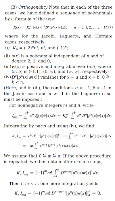
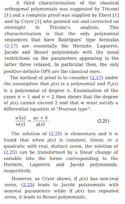
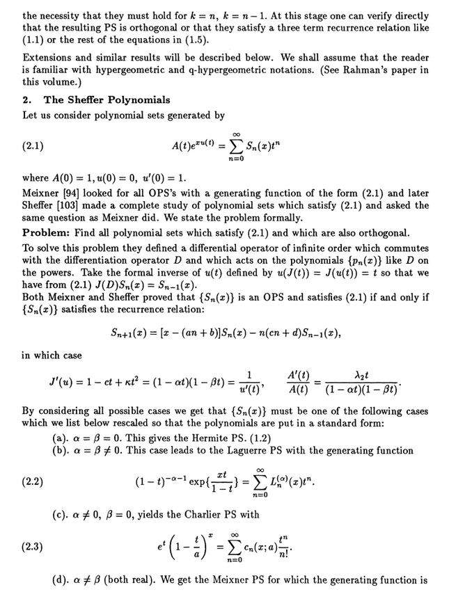
{$\{P_n(x)\}$} is a Sheffer orthogonal polynomial set iff it satisfies the recurrence relation, as per Galiffa and Riston:

{$$P_{n+1}(x) = (x + c_1 + c_2n)P_n(x) - (c_3n+c_4n^2)P_{n-1}(x)$$}

{$$P_{n+1}(x) = (x + (\alpha + b) + bn)P_n(x) - ((c+d)n+d n^2)P_{n-1}(x)$$}

{$$P_{n+1}(x) = (x + a_1 + 2h_2n)P_n(x) - ((a_1^2 - 2a_2 + 2a_1h_2-4h_2^2+3h_3)n+(4h_2-3h_3)n^2)P_{n-1}(x)$$}

And compare this with the recurrence relation given by Kim and Zeng:

{$$P_{n+1}(x)=[x-(\alpha_{KZ}\beta_{KZ} + (u_3 + u_4)n)]P_n(x)-n(\beta_{KZ} + n - 1)u_1u_2P_{n-1}(x)$$}

where, in the moments, whose terms are permutations, {$\alpha_{KZ}$} counts fixed points, {$\beta_{KZ}$} counts the number of cycles, {$u_1$} counts ascents-descents (peaks), {$u_2$} counts descents-ascents (valleys), {$u_3$} counts ascents-ascents, {$u_4$} counts descents-descents.

I set my notation {$f=\alpha_{KZ}\beta_{KZ}$}, {$l=u_3+u_4$}, {$k=u_1u_2$}, {$\gamma=\beta_{KZ}u_1u_2$} we get, in my notation:

{$$P_{n+1}(x)=[x-(ln+f)]P_n(x)-(n(n-1)k + n\gamma)P_{n-1}(x)$$}

Note that {$u_3$} and {$u_4$} only appear as the sum {$u_3+u_4$} and that {$u_1$} and {$u_2$} only appear as the product {$u_1u_2$} so they are underdetermined. We thus have a lot of leeway as to how we define {$u_1$}, {$u_2$}, {$u_3$}, {$u_4$}. So we can define them as {$\alpha = u_1 = u_3$} to be the weight attributed to each ascent and {$\beta = u_2 = u_4$} to be the weight attributed to each descent.

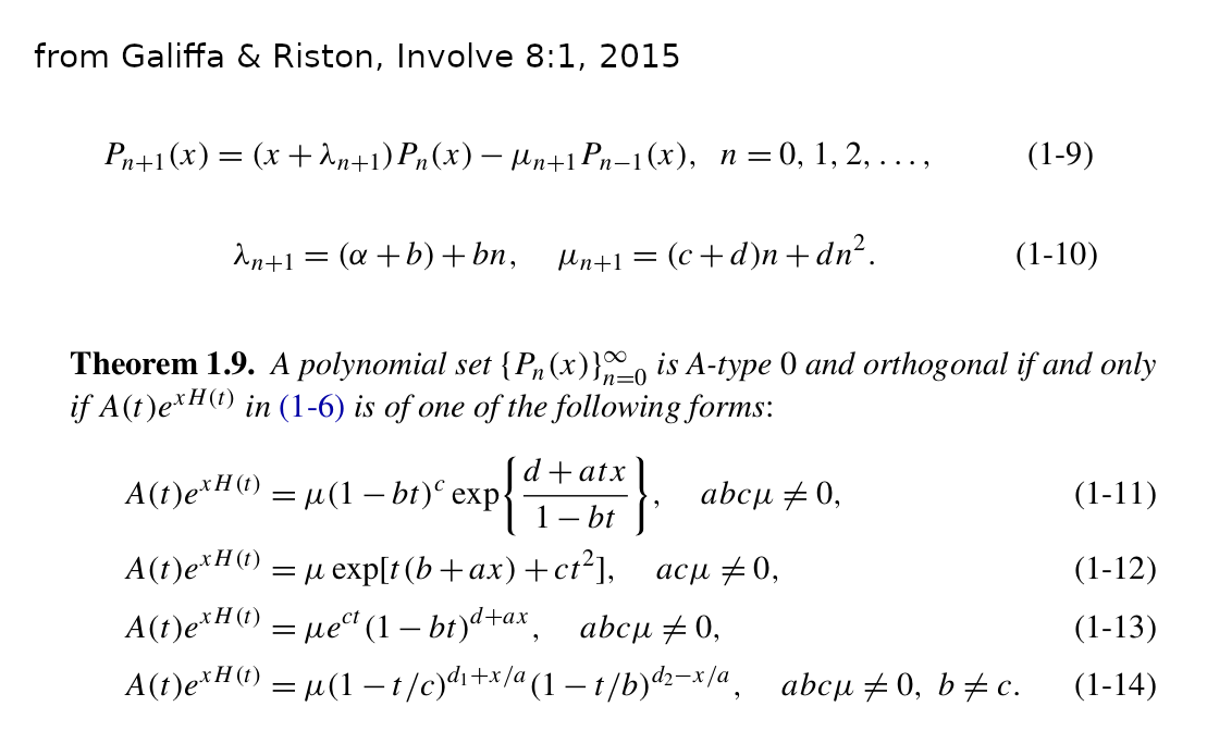
As shown by Galiffa and Riston, the recurrence relation is determined by {$a_1$}, {$a_2$}, {$u_2$}, {$u_3$}. Namely,

{$f=-a_1$}, {$l=-2h_2$}, {$\gamma=a_1^2-2a_2+2a_1h_2$}, {$k=4h_2^2-3h_3$}

We can turn these equations around to give combinatorial meaning to the initial terms of {$A(t)$} and {$u(t)$}.

{$a_1 = -f$}, {$a_2 = \frac{f^2+fl-\gamma}{2}$}, {$h_2=\frac{-l}{2}$}, {$h_3=\frac{l^2-k}{3}$}.

We can suppose {$f=0$} by considering the translation of {$x$} to {$(x-f)$}. Then {$a_2=\frac{-\gamma}{2}$}. This yields:

{$$A(t)=1 - \frac{\gamma}{2}t^2 + a_3t^3 + a_4t^4 + \cdots$$}

{$$u(t)=t - \frac{l}{2}t^2 + \frac{l^2-k}{3}t^3 + u_4t^4 + \cdots$$}

Note that the higher order terms are not relevant, in that they are determined by the initial terms.

Then we get the most natural and profound expressions for {$u'(t)$} and {$A'(t)$}.

{$A'(t) = - \gamma t + \textrm{echo terms}$}

{$u'(t) = 1 - lt + (l^2-k)t^2 + \textrm{echo terms}$}

Alternatively, factoring {$1+lt+kt^2=(1-\alpha t)(1-\beta t)$}, we have {$l=(-\alpha)+(-\beta)$} and {$k=(-\alpha)(-\beta)$}. Thus we have

{$$u'(t) = 1 -(\alpha + \beta) t + (\alpha^2 + \alpha\beta + \beta^2)t^2 + \textrm{echo terms}$$}

I mean by "echo terms" that the higher order terms are completely determined by the initial terms and have no independent significance.

Note that we can interpret {$l$} to mean {$\textrm{NAND(A,B)}$}, for (NOT (A AND B) = (NOT A) OR (NOT B), and we can interpret {$k$} as {$\textrm{NOR(A,B)}$}, for (NOT (A OR B) = (NOT A) AND (NOT B). NAND and NOR are the two logical operators from which all other operators can be derived. And algebraically, we get an interesting logic where NAND(A,B) = (-A)(-B) = AB = AND(A,B). I should study this logic.

It is meaningful to focus on {$xP_n(x)$} and thus contemplate the following expression:

{$$xP_n(x) = P_{n+1}(x) + (nl + f) P_n(x) + n(nk + c) P_{n-1}(x)$$}

Calculating the coefficients of {$h(t)$} and {$A(t)$}

The combinatorics of the orthogonal Sheffer polynomials is dictated by two constraints. They are Sheffer polynomials, which makes them space builders, in that each new polynomial adds a point in space. And they are orthogonal, which means that multiplying a polynomial {$P_n(x)$} by {$x$}, which is to say, {$xP_n(x)$}, is expressed in terms of three polynomials: {$P_{n+1}(x)$}, {$P_n(x)$}, {$P_{n-1}(x)$}. Orthogonality gives the paths on the space, and those paths relate a space to that with one point more and one point less. And what does {$x$} mean by itself? And what does it mean to multiply {$x$}, for example, by {$P_n(x)$}?

Calculating the Sheffer polynomials as space builders, we can see that the coefficients are given by the nth derivatives with regard to {$t$}, evaluated at {$t=0$}. {$a_i = \frac{\textrm{d}^i}{\textrm{dt}^i}A(t)|_{t=0}$} and {$h_i = \frac{\textrm{d}^i}{\textrm{dt}^i}h(t)|_{t=0}$}.

Once we impose the recursion relation, we can make use of the coefficients of that relation, which have combinatorial meaning as weights for paths in space. We can apply the recursion relation to {$P_{-1}=0$} and to {$P_{0}=1$} and upwards to get values for all {$P_n(x)$} in terms of those weights. Then we can express the coefficients of {$P_n(x)$} in two ways, to relate the coefficients / derivatives / compartments {$a_i$} and {$h_i$} and the weights {$l, k, f, \gamma$} for paths.

We know that {$a_it^i$} is the constant term in {$P_i(x)t^i$} because any contribution from {$xh(t)$} would carry an {$x$} and it is the only term with {$t^i$} in {$A(t)$}.

Note that the definition of {$P_n(x)$} as a Sheffer polynomial is nonmonic, whereas the recurrence relation, as written, makes it monic, and so the results are distinguished by a multiplicative factor of {$n!$}. Note also that the recurrence relation has coefficients that depend on {$n$} and {$n(n-1)$} and that these are to be divided by {$n$}. This means that we actually have constant factors {$\frac{n}{n}=1$} and additional growth factors {$\frac{1}{n}$} and {$n-1$}.

The first few values are:

{$a_0 = 1$}
{$a_1 = -f$}
{$2!a_2 = lf + f^2 - g$}
{$3!a_3 = - 2l^2f - 3lf^2 + 2lg - f^3 + 2fk + 3fg$}
{$4!a_4 = 9l^3f + 15l^2f^2 - 9l^2g + 7lf^3 - 24lfk - 18lfg + f^4 - 12f^2k - 7f^2g + 6kg + 3g^2$}
{$5!a_5 = - 27l^4f - 54l^3f^2 + 27l^3g - 36l^2f^3 + 90l^2fk + 72l^2fg - 10lf^4 + 84lf^2k + 51lf^2g - 36lkg - 18lg^2 - f^5 + 18f^3k + 10f^3g - 36fk^2 - 48fkg - 15fg^2$}

The number of terms grows as: 1, 3, 6, 11, 17, 26, 36, 50... This is the sequence A003453 which counts the number of nonequivalent dissections of an n-gon into 3 polygons by nonintersecting diagonals up to rotation and reflection. It may also be related to A005744 which counts the number of n-covers of a 2-set.

And the supposed number of objects (assuming no objects are cancelling away) grows as: 1, 3, 13, 111, 633, 3531. But there is no related sequence.

Note that as regards the recurrence relation, the difference between the terms {$a_i$} and {$h_i$} is whether or not they are picking up the {$x$} in the term {$[x-(ln+f)]$}. We can set {$x=0$} to see how we build up the terms for {$a_i$}. Really, the analysis of this algorithm should be done for {$\mu_i$} and {$\lambda_i$} and should give what Viennot has already gotten for the general case of the orthogonal polynomials in terms of walks. And then I can consider what happens when we specialize to {$n,l,f,k,\gamma$}.

Causal chains

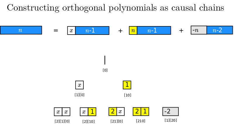
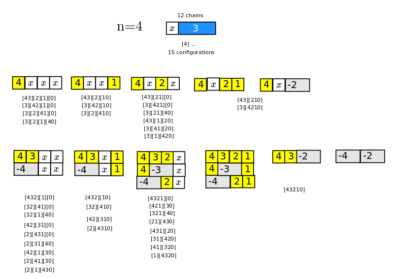
I am studying the terms generated by the recurrence relation {$P_{n+1}(x)=(x + L_{n+1})P_n(x) - M_{n+1}P_{n-1}(x)$}. Note that the values {$L_{n+1}$} and {$M_{n+1}$} can depend on {$n+1$} in a most arbitrary way.

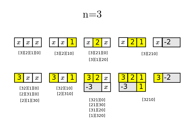
The combinatorics is straightforward. Repeated iteration yields an interpretation of {$P_{n+1}(x)$} as one-dimensional causal chains made of three kinds of blocks laid side by side. There is a block of length 1 and weight {$x$}, a block of length 1 and weight {$L_{i+1}$}, and a block of length 2 and weight {$-M_{i+1}$}.

The number of terms grows as 1, 2, 5, 12, 29, 70, 169, 408 These are the Pell numbers {$P_n= \frac{(1+\sqrt{2})^n - (1-\sqrt{2})^n}{2\sqrt{2}}$} used for approximating the square root of 2. Also, the numbers {$(\frac{P_{2n}}{2})^2$} are the square triangular numbers. The recurrence relations for the Pell numbers {$P_{n+1}=2P_{n}+P_{n-1}$} are very similar to that of the Fibonacci numbers {$F_{n+1}=2F_{n}+F_{n-1}$}. Indeed, the terms without {$x$} are counted by the Fibonnaci numbers. The Pell numbers are smaller than the Bell numbers, which grow as 1,2,5,15,52...

Deriving the differential equations

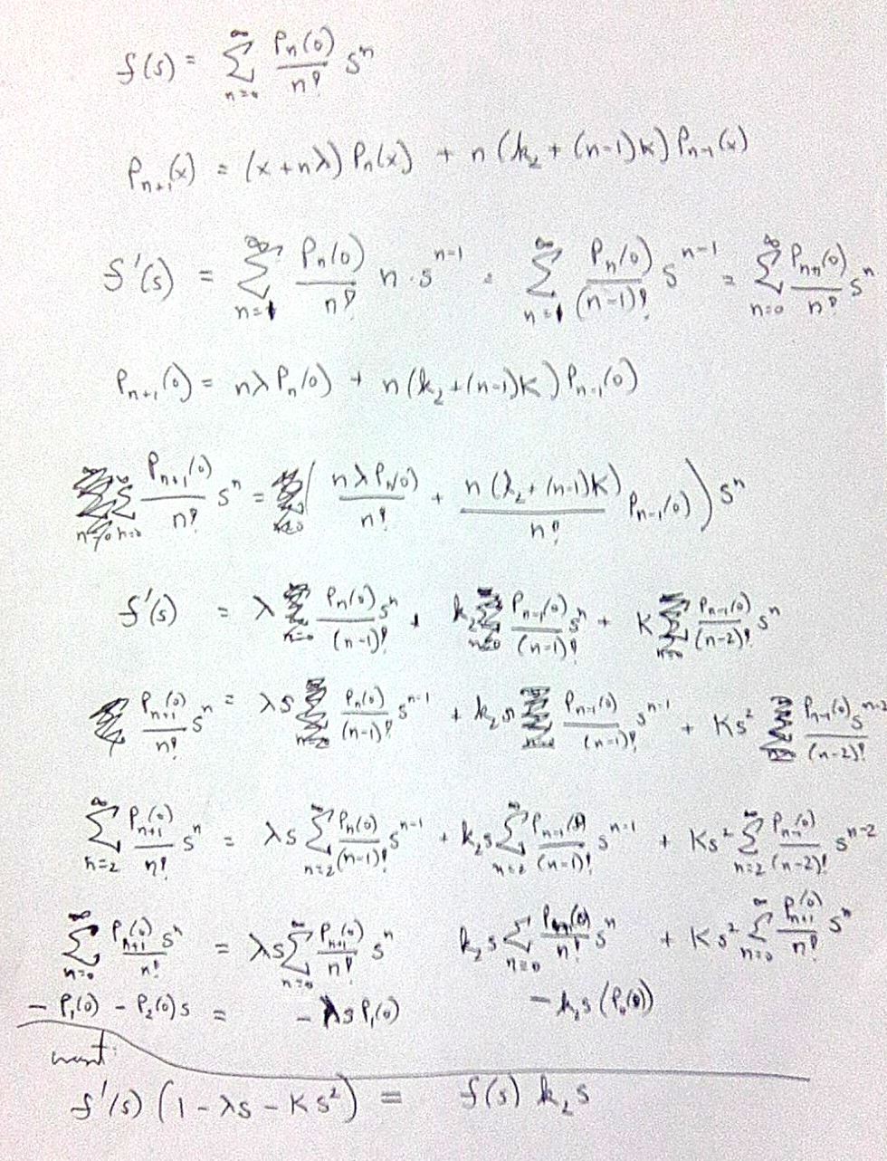
Here are my notes for deriving the differential equation relating {$A(t)$} and {$A'(t)$}. Apparently, this is essentially the same as the differential equation relating {$f(s)=\sum_{n=1}^{\infty}\frac{P_n(0)}{n!}s^n$} and {$f'(s)=\sum_{n=0}^{\infty}\frac{P_{n+1}(0)}{n!}s^n$}. The idea is to sum over the recurrence relation and then identify {$f(s)$} and {$f'(s)$}, place them on either side, and divide. The initial terms of the series yield a constant, but fortunately that constant is {$0$}.

For {$u'(t)$} it is important to appreciate that {$u'(t)=\frac{\textrm{du}}{\textrm{dt}}$} and so

{$$t'(u)=\frac{\textrm{dt}}{\textrm{du}}=\frac{1}{u'(t)}$$}

Differential equations

{$\{P_n(x)\}$} is an orthogonal polynomial set iff {$u(t)$} and {$A(t)$} satisfy the differential equations where {$(1-\alpha t)(1-\beta t)=1+lt+kt^2$} is a polynomial with real coefficients but possibly complex roots:

{$$u'(t)=\frac{1}{(1-\alpha t)(1-\beta t)}=\frac{1}{1+lt+kt^2}=\frac{A'(t)}{-(c+k)tA(t)}=\frac{A'(t)}{\gamma tA(t)}$$}

Here {$A(t)=\sum_{n=0}^{\infty}\frac{P_n(0)}{n!}t^n$}.

Thus, given a choice of steps {$\alpha$} and {$\beta$}, a link {$l$} expresses "or" {$-(\alpha + \beta)$} with a negative weight, and a kink {$k$} expresses "and" {$\alpha\beta$}.

What is the meaning of {$c+k$}?

I should read Differential equation and learn more about them. I can also study Bachioua Lahcene. On Pearson families of distributions and its applications.

Here the classification is a straightforward analysis of the possibilities for {$u'(t)$}:

polynomials	{$\alpha$}, {$\beta$}	{$u'(t)$}	{$u(t)$}
Hermite	{$\alpha=\beta$}, {$\beta=0$}	{$1$}	{$t$}
Charlier	{$\alpha\neq\beta$}, {$\beta=0$}	{$\frac{1}{1-\alpha t}$}	{$-\frac{1}{\alpha}\textrm{ln}(1-\alpha t)$}
Laguerre	{$\alpha=\beta$}, {$\beta\neq 0$}	{$\frac{1}{(1-\alpha t)^2}$}	{$\frac{t}{(1 - \alpha t)}$}
Meixner	{$\alpha \neq \beta$}, both real, nonzero	{$\frac{1}{(1-\alpha t)(1-\beta t)}$}	{$\frac{1}{\beta - \alpha}\textrm{ln}(1-\alpha t)+\frac{1}{\alpha - \beta}\textrm{ln}(1-\beta t)$}
Meixner-Pollaczek	{$\alpha=\overline{\beta}$}, complex conjugates, nonzero	{$\frac{1}{(1-\alpha t)(1-\overline{\alpha} t)}$}	{$\frac{1}{\overline{\alpha} - \alpha}\textrm{ln}(1-\alpha t)+\frac{1}{\alpha - \overline{\alpha}}\textrm{ln}(1-\overline{\alpha} t)$}
Incorrect Meixner-Pollaczek	{$\alpha=\overline{\beta}$}, complex conjugates, nonzero	{$\frac{1}{1 + \|\alpha\|^2t^2}$}	{$\frac{1}{\|\alpha\|}\textrm{tan}^{-1}\|\alpha\|t$}

Note that {$u(0)=0$} determines the constant of integration. For the Laguerre polynomials, it is {$-\frac{1}{\alpha}$}, and in every other case it is {$0$}.

We have the Taylor series expression {$-\textrm{ln}(1-\alpha t)=\alpha t - \frac{1}{2}\alpha^2t^2 + \frac{1}{3}\alpha^3t^3 - \frac{1}{4}\alpha^4t^4 +\cdots$}. The most general generating function is for the Meixner polynomials:

{$$\frac{1}{\beta - \alpha}(\textrm{ln}(1-\alpha t) - \textrm{ln}(1-\beta t)) = -t + \frac{1}{2}t^2(\alpha+\beta)-\frac{1}{3}t^3(\alpha^2+\alpha\beta+\beta^2) + \frac{1}{4}t^4(\alpha^3+\alpha^2\beta+\alpha\beta^2+\beta^3)+\cdots$$}

On the right hand side, I have cancelled {$\beta - \alpha$} from the numerator and denominator. From the resulting generating function I can derive the cases for the Hermite, Charlier and Laguerre cases. But so far I don't see how I can get the Meixner-Pollaczek generating function by setting {$\beta=\overline{\alpha}$}.

polynomials	{$\textrm{ln}A(t)$}	A(t)	{$e^{xu(t)}$}
Hermite	{$\frac{1}{2}\frac{\gamma}{\alpha ^2}(\alpha t)^2$}	{$(e^{\frac{1}{2}(\alpha t)^2})^{\frac{\gamma}{\alpha^2}}$}	{$(e^{\alpha t})^{\frac{x}{\alpha}}$}
Charlier	{$\frac{\gamma}{\alpha^2}[\alpha t - \textrm{ln}(1-\alpha t)]$}	{$(\frac{e^{\alpha t}}{(1-\alpha t)})^{\frac{\gamma}{\alpha^2}}$}	{$(\frac{1}{1-\alpha t})^{\frac{x}{\alpha}}$}
Laguerre	{$\frac{\gamma}{\alpha^2}[\textrm{ln}(1-\alpha t)+\frac{\alpha t}{1-\alpha t}]$}	{$((1-\alpha t)e^{(\frac{\alpha t}{1 - \alpha t})})^{\frac{\gamma}{\alpha^2}}$}	{$(e^{\frac{\alpha t}{(1 - \alpha t)}})^{\frac{x}{\alpha}}$}
Meixner	{$\frac{\gamma}{\alpha \beta}[\frac{\alpha}{\alpha - \beta} \textrm{ln}(1-\beta t) - \frac{\beta}{\alpha - \beta} \textrm{ln}(1 - \alpha t)]$}	{$(\frac{(1-\beta t)^\alpha}{(1-\alpha t)^\beta})^{\frac{\gamma}{\alpha\beta(\alpha - \beta)}}$}	{$(\frac{1-\beta t}{1-\alpha t})^{\frac{x}{\alpha-\beta}}$}
Meixner-Pollaczek	{$\frac{\gamma}{\alpha \overline{\alpha}}[\frac{\alpha}{\alpha - \overline{\alpha}} \textrm{ln}(1-\overline{\alpha} t) - \frac{\overline{\alpha}}{\alpha - \overline{\alpha}} \textrm{ln}(1 - \alpha t)]$}	{$(\frac{(1-\overline{\alpha} t)^\alpha}{(1-\alpha t)^\overline{\alpha}})^{\frac{\gamma}{\alpha\beta(\alpha - \overline{\alpha})}}$}	{$(\frac{1-\overline{\alpha} t}{1-\alpha t})^{\frac{x}{\alpha-\overline{\alpha}}}$}
Incorrect Meixner-Pollaczek	{$\frac{\gamma}{2\|\alpha\|^2}\textrm{ln}(1+\|\alpha\|^2t^2)$}	{$(\sqrt{1+\|\alpha\|^2t^2})^{\frac{\gamma}{\|\alpha\|^2}}$}	{$(e^{\textrm{tan}^{-1}\|\alpha\|t})^{\frac{x}{\|\alpha\|}}$}

The Meixner generating function can be written:

{$$(\frac{1}{1-\alpha t})^{\frac{1}{\alpha-\beta}(\frac{\gamma}{\alpha}+x)}(\frac{1}{1-\beta t})^{\frac{1}{\beta-\alpha}(\frac{\gamma}{\beta}+x)}$$}

I suppose this is the most general form from which the others can be specialized.

I'm curious how this relates to the Jacobi polynomials, whose weight {$(1-x)^a(1+x)^b$} seems very much related to this expression.

Compare with Galiffa & Riston

I studied how the variables {$a$}, {$b$}, {$c$}, {$d$} that Galiffa & Riston use in their recurrence relation appear in their generating functions. But it seems to me, upon inspection, that they aren't the same variables, unfortunately.

polynomials	{$h_2$}, {$h_3$}	kinks {$k$}, links {$l$}
Hermite	{$h_2^2=h_3=0$}	{$k=0$}, {$l=0$}
Charlier	{$h_2^2=\frac{3}{4}h_3$}	{$k=0$}, {$l\neq 0$}
Laguerre	{$h_2^2=h_3$}	{$l^2-4k=0$}
Meixner	{$h_2^2>h_3$}	{$l^2-4k>0$}
Meixner-Pollaczek	{$h_2^2<h_3$}	{$l^2-4k<0$}

Note that in the Meixner-Pollaczek case we have {$\alpha=a+bi$} and {$|\alpha|=a^2+b^2$} and we are dealing with a circle, as with {$\textrm{tan} \theta$}. What is the meaning of {$\textrm{tan}^{-1}$}?

Compare with the Pearson system for classifying distributions as solutions to the differential equation

{$$\frac{\textrm{dy}}{\textrm{dx}} = \frac{y(m-x)}{a+bx+cx^2}$$}

Viennot's Combinatorial Interpretation

Relating the five cases

Understand how the various cases relate to each other, for example, in taking limits, or in perturbing degeneracies in ways so that they are nondegenerate.

Further steps

Further steps I can take...

I will write to India to ask how to contact Xavier Viennot and who is working on related combinatorics.
How can I relate Zeng's interpretation of {$P_n(x)$} with pairs of combinatorial interpretations for {$A(t)$} and {$e^{xu(t)}$}?
Learn about the Pearson system of distributions.
Explore what happens when we successively integrate {$\textrm{ln} x$}.

Sources

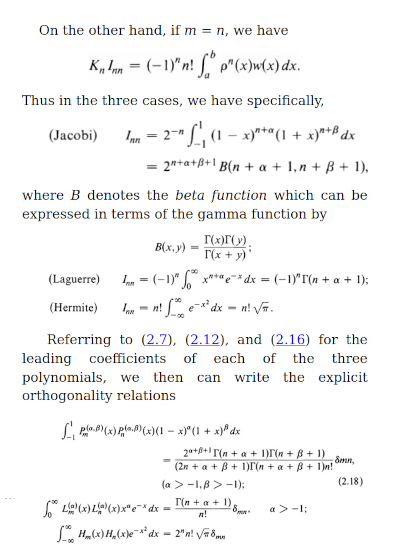
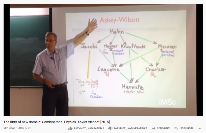
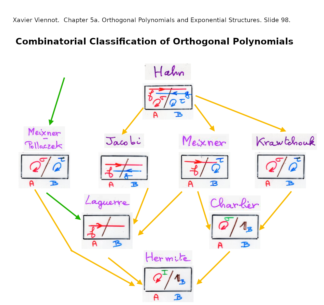
Theodore Chihara. An Introduction to Orthogonal Polynomials. 1978.

Xavier Viennot overviews the combinatorics of the moments of orthogonal polynomials: Hermite (involutions), Laguerre (permutations), Charlier (partitions), Meixner (ordered partitions), Meixner-Pollaczek (secant = even alternating permutations), Chebyshev I (ways of choosing half), Chebyshev II (Catalan).